Drawing on the Logarithmic Scale

import sympy
from sympy import symbols, diff, ln
from sympy.codegen.cfunctions import log2
import functools
import matplotlib.pyplot as plt

x0=symbols("x0")
x1=symbols("x1")

def call(f, x):
    return f(x)

def mapv(a, b):
    return list(map(a, map(lambda x: 1.0 * x, b)))

def mapv_indexed(f, coll):
    return list(map(lambda x: [x, f(x)], map(lambda x: 1.0 * x, coll)))

class PipeAsCall(object):
    def __init__(self, func):
        self.func = func
    def __or__(self, other):
        return self.func(other)
    def __call__(self, x):
        return self.func(x)

class Transducer(PipeAsCall):
  pass

def partial(*args):
    return PipeAsCall(
        functools.partial(*args))

def D(f):
  var = symbols("var")
  return PipeAsCall(sympy.lambdify([var], diff(f(var), var), "sympy"))

def rnd(expr):
     return expr.xreplace({n: round(n, 3) for n in expr.atoms(sympy.Number)})

def plot(f, x):
    if (type(f)==str) or (type(f)==sympy.core.numbers.Float):
       return "That's not something you can plot"
    else:
       plt.plot(x, mapv(f, x), "o")

def plotting(f):
    if type(f) == Transducer:
        return partial(lambda f, coll: plt.plot(list(map(lambda x: x[0],f(coll))),list(map(lambda x: x[1],f(coll))), "o"), f)
    else:
        return partial(lambda f, x: plt.plot(x, mapv(f, x), "o"), f)

isPositive = lambda n: True if n>0 else False

def smaller(x):
    return lambda n: True if n<x else False

def filtering(f):
    return Transducer(functools.partial(lambda f,coll: list(filter(f, coll)), f))

def mapping(f):
    return Transducer(functools.partial(mapv_indexed, f))

def compose(f, g):
    return Transducer(lambda x: f(g(x)))

frequencies = [16.35, 17.32, 18.35, 19.45, 20.6, 21.83, 23.12, 24.5, 25.96, 27.5, 29.14, 30.87, 32.7, 34.65, 36.71, 38.89, 41.2, 43.65, 46.25, 49.0, 51.91, 55.0, 58.27, 61.74, 65.41, 69.3, 73.42, 77.78, 82.41, 87.31, 92.5, 98.0, 103.83, 110.0, 116.54, 123.47, 130.81, 138.59, 146.83, 155.56, 164.81, 174.61, 185.0, 196.0, 207.65, 220.0, 233.08, 246.94, 261.63, 277.18, 293.66, 311.13, 329.63, 349.23, 369.99, 392.0, 415.3, 440.0, 466.16, 493.88, 523.25, 554.37, 587.33, 622.25, 659.25, 698.46, 739.99, 783.99, 830.61, 880.0, 932.33, 987.77, 1046.5, 1108.73, 1174.66, 1244.51, 1318.51, 1396.91, 1479.98, 1567.98, 1661.22, 1760.0, 1864.66, 1975.53, 2093.0, 2217.46, 2349.32, 2489.0, 2637.0, 2793.83, 2959.96, 3135.96, 3322.44, 3520.0, 3729.31, 3951.0, 4186.0, 4434.92, 4698.63, 4978.0, 5274.0, 5587.65, 5919.91, 6271.93, 6644.88, 7040.0, 7458.62, 7902.13]

import numpy as np
import json
import inspect

# https://muted.io/note-frequencies/
data = np.genfromtxt('notes.txt', delimiter='\t', dtype=str)
row_names = data[:, 0].tolist()
numerical_data = np.matrix.transpose(data[:, 1:]).astype(float).tolist()

nofreq = [item
    for subl in
      [list(map(lambda n,f: [n, idx, f], row_names, fs))
        for idx, fs in enumerate(numerical_data)]
   for item in subl]

frequencies = [n[2] for n in nofreq]

print("<script>")
print("statejs['notenames']= ")
print(json.dumps(row_names))
print("statejs['frequencies']= ")

print(json.dumps([[nf[0] + str(nf[1]), nf[2]] for nf in nofreq if not nf[0].endswith("s")]))
print("</script>")

# instead of using the plain js
# print("<script src='jsfiles/notes.js'></script>")
# we load the respective Scittle code

print("<script>")
with open('notes.cljs', 'r') as file:
    data = file.read().replace('\n', '')
print("scittle.core.eval_string('", data, "')")
print("</script>")

1

A B C D E F

The musical scale is logarithmic – I am going to use this concrete example to show my way of doing mathematical plots.

_

2

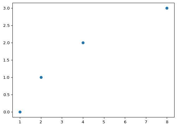
The curve above is drawn using the log2. To show this specific plot, I had to make some choice for the scale factors. – This notebook is online at the following address

https://kloimhardt.github.io/site/log.html

Its appendix links a Jupyter notebook for the ensuing code snippets. But I have jumped ahead. My story starts with the Python language. And plotting just the plain log2. And that already hits upon the main message of my presentation.

_

print("<script>")
with open('log23.cljs', 'r') as file:
    data = file.read().replace('\n', '')
print("scittle.core.eval_string('", data, "')")
print("</script>")

3

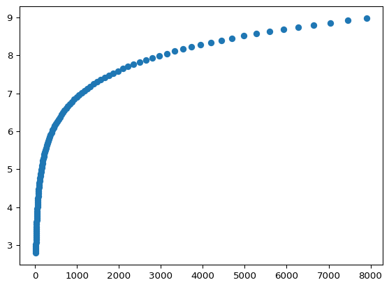
plot(log2, [1, 2, 4, 8])

The message is this. – It is the log2 that you plot. This is so obvious that I’d like to state what log2 is not. It is not the log2 of x or y or z. Also, it is not some text that contains the string log2. Rather, log2 is a mathematical object. Only objects like this are suitable for plotting within the paradigm of my presentation.

_

4

A B

I am aware that you need some time for digesting my self-imposed plotting restrictions. So I move more towards the practical goal. -B- I need to get more to something like this. For that, I need to get back to the formula I showed at the start.

_

5

A C D E

The formula I showed at the start is not something you can plot. -B- This is the main theme again. The theme is that I need a proper mathematical target to plot. To arrive at such a target, it is necessary to bind the formula to a procedure. -C- The procedure itself I gave the name Poe. It takes three arguments. Two parameters and the frequency x. -D- The procedure does the wanted computation. – It returns the value given by the formula. -E- In its code, you have to replace the numbers with the names of the two parameters. – I provide the procedure as Python code. -F-

_

B

plot("log2(x / 220) * 7", [1, 2, 4, 8])

"That's not something you can plot"

F

def Poe(intersect, steps, x):
    return log2(x/intersect) * steps

Poe(220, 7, 440)

\(\displaystyle 7.0\)

6

A B D F I can plot log2 because it is a mathematical object. -B- But still I cannot plot the procedure Poe. -C- I need an operation called “partial” to transform Poe into the proper target to plot. -D- The procedure named “partial” takes “Poe” as an argument. – Then I can perform the plotting. -E- Here is the main theme in spades: “partial” taking a procedure to deliver the target to plot. -F- I turn all this into yet another procedure named log2b – That is very convenient for plotting. -G-

def log2b(intersect, steps):
    return partial(Poe, intersect, steps)

_

C

plot(Poe(220, 7, 440), [1, 2, 4, 8])

"That's not something you can plot"

E

plot(partial(Poe, 220, 7), [1, 2, 4, 8])

G

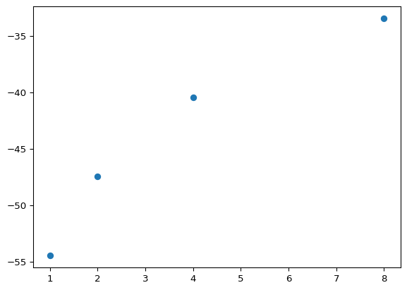
plot(log2b(220, 7), [1, 2, 4, 8])

7

A B D F G

Not only can log2b be plotted. -B- Log2b can also be called. -C- Not only can log2b be called with data of type number. Log2b can also be called with a symbol. -DE- Using symbols along with numbers is possible thanks to a package named Sympy. Here you see that for the name of the symbol I chose x-naught. But x-naught is only the default of possible choices. As a symbol, for example, I can also choose x1. -F- For log2b, the x1 is just yet another data that happens to be of type symbol. This idea of “symbols as data” is the source for my freedom of choice. Before being able to process some data, log2b needs to be initialized with two parameters. -G- But these do not need to be of type integer. The float 0.7 does nicely as well. -a-

_

C

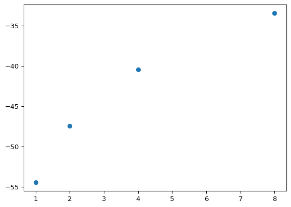
call(log2b(220, 7), 8)

\(\displaystyle -33.4695179946726\)

E

call(log2b(220, 7), x0)

\(\displaystyle 7 \operatorname{log}_{2}{\left(\frac{x_{0}}{220} \right)}\)

a

call(log2b(1, 0.7), x1)

\(\displaystyle 0.7 \operatorname{log}_{2}{\left(x_{1} \right)}\)

8

A B C D E F G

I would not have bothered you with my O point seven invention, hadn’t I discovered it to be a segue to the natural logarithm. -B- In general, you can fit a series of triangles onto any curve. -C- Moving those triangles to the ground level reveals -D- that a new curve “one over x” fits their heights quite agreeably. −E− You can also try the other way around -F- That does not work quite as well. -G- The trick is to shrink the area while retaining the angles.

_

9

A D

I hope my triangles just formed an agreeable entertainment. For me they were (while making them). In conclusion, I assume you caught on to the topic I am aiming at: -D- differentiation. – Taking the derivative of log2b is simple and easy.

_

10

call(D(log2b(1, 0.7)), x0).evalf()

\(\displaystyle \frac{1.00988652862227}{x_{0}}\)

call(D(ln), x0)

\(\displaystyle \frac{1}{x_{0}}\)

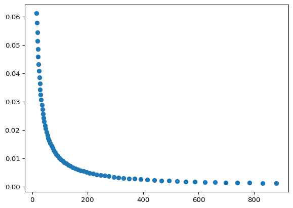
With the log2b initialized at O point seven, I calculate its derivative. As a result I almost get one over x. To become exact, I need to switch to “ln”, the natural logarithm. The pictures above can, within this presentation, be called its pinnacle. As a kind of confirmation, I’d like to drop some names. In math, the procedure named “call” is a functional while D is an operator. In computer science, both is called functions of higher order. The natural logarithm “ln” of course is a function in any field.

_

–

\[\Large \left. \frac{d \ln(x)}{dx} \right|_{x=x_0}\]

I’d like to wind down with a note on notation. When I differentiate a function like “ln” and then evaluate that derivative at x-naught, the common notation is the vertical bar. This bar is also called “pipe”.

_

–

A B

In taking this inspiration from math, I use pipe in my pictures as well. -B- Note: it’s not the D operator which is replaced by the pipe, but it’s the “call” that is dropped. – Not only can “pipe” be used in pictures. The pipe can also be used within Python code. -C- You might think that my notation for pipe is hard to achieve. This is not so. My custom pipe is a few lines of Python only. – The pipe symbol is an invented alternative notation. In the following finale, I’d like to discover its explanatory virtues.

_

C

(D(ln) | x0)

\(\displaystyle \frac{1}{x_{0}}\)

–

class PipeAsCall(object):
    def __init__(self, func):
        self.func = func
    def __or__(self, other):
        return self.func(other)
    def __call__(self, x):
        return self.func(x)

def partial(*args):
    return PipeAsCall(
        functools.partial(*args))

11

A B C E G b

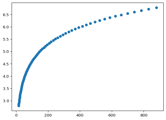
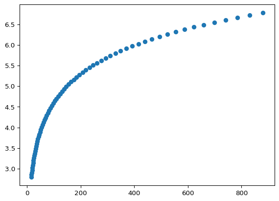
The pipe notation is very versatile. I can also use it when plotting something. -B- In my dataset, the highest frequency is eight kilohertz. -CD- I’d like to cut that down to 900 cycles per second. -E- So I apply a filter – and plot. -F- I want to move the filtering to the left. Or in a more picturesque manner: I want the filtering to be ahead of the pipes. For this, I use function composition. -G- This composition is completely decoupled from input sources and output formats. This leads to a method commonly known as “transducing” – Transducers are ahead of the pipe. -a- For sure you can insert differentiation into the composition as easily as ever. -bc-

_

D

(plotting(ln) | frequencies)

F

(plotting(ln) |
  (filtering(smaller(900)) |
    frequencies))

a

(plotting
  (compose
    (mapping(ln), 
     filtering(smaller(900)))) |
  frequencies)

c

(plotting
  (compose
    (mapping(D(ln)), 
     filtering(smaller(900)))) |
  frequencies)

Appendix

Try the Jupyter notebook:

• go to the Jupyter-lite web page https://jupyter.org/try-jupyter/lab/
• click File -> Open from URL
• paste the following URL: https://raw.githubusercontent.com/kloimhardt/site/main/mysite/log.ipynb
• select the “Pyodide” Kernel and click Run -> Run All Cells

This notebook was generated using Quarto.

• Walkthrough video for the notebook: https://www.youtube.com/watch?v=FE5pB3yvCRs
• The source code can be viewed here: https://github.com/kloimhardt/site/blob/main/mysite/log.qmd

The idea for this Python notebook is based on an older interactive workspace:

• Watch the Clojure visual-tools meeting from 2022
• Try out the workspace at https://kloimhardt.github.io/cljtiles.html?page=FDG001
• Maybe also try https://kloimhardt.github.io/cljtiles.html?page=116